Using percent vectors

Let’s start by loading the phsmethods package.

library(phsmethods)

Motivation

Working with percentages in R can be frustrating, to say the least. A typical workflow for generating percentages might look like this:

Generate proportions
Scale up proportions to percentages (multiplying by 100)
Round percentages
Convert percentages to characters
Append a percentage symbol
Use proportions for math operations and rounding
Use formatted percentage strings for outputs

With <percent> vectors, this workflow is reduced to:

Generate proportions
Convert to percentages

This is clearly much simpler and allows for cleaner and more reproducible code.

Creating percentages

The primary function for converting to percentages is as_percent(). This converts a <numeric> vector to a <percent> vector, handling the formatting and rounding when needed, i.e printing or converting to a character vector.

(p <- as_percent(0.055))
#> [1] "5.5%"

Internally, the numeric vector is left as-is, which can be confirmed by examining the vector via unclass(x).

unclass(p)
#> [1] 0.055
#> attr(,".digits")
#> [1] 2

The only time percentage formatting actually happens is when the <percent> vector is printed or converted to a character vector (via as.character or format).

print(p)
#> [1] "5.5%"
as.character(p)
#> [1] "5.5%"
format(p)
#> [1] "5.5%"

Rounding

Percentages are rounded using a round-halves-up approach. The rationale for straying away from R’s round-to-even is that readers generally expect percentages to be rounded this way in formatted outputs such as papers, reports, etc. We are less concerned with statistical bias and more concerned with formatting.

There are two main ways to control how percent vectors are rounded:

Rounding via `as_percent` + `digits`

as_percent does two things:

It creates a <percent> vector
It sets the “.digits” attribute, which controls how the percent vector is printed downstream.

p2 <- as_percent(p, digits = 0)

# Prints and formats to 0 decimal places
print(p2)
#> [1] "6%"
as.character(p2)
#> [1] "6%"

# Underlying data has not been rounded!
unclass(p2)
#> [1] 0.055
#> attr(,".digits")
#> [1] 0

Rounding via `round()`

This method will ‘physically’ round the numbers.

p3 <- round(p, digits = 0)

p3
#> [1] "6%"

# Underlying data has been rounded
unclass(p3)
#> [1] 0.06
#> attr(,".digits")
#> [1] 2

In practice, this means that rounding with as_percent is more flexible as it reduces downstream errors that can accumulate from premature rounding.

Math with percent vectors

A strong feature of <percent> vectors is the ability to use them in mathematical contexts without extra unnecessary work.

# Helper to create literal percentages
percent <- function(x) {
  as_percent(x / 100)
}

Addition, subtraction, multiplication and division.

percent(50) + percent(25) # = 50% + 25% = 75%
#> [1] "75%"
percent(50) - percent(25) # = 50% - 25% = 25%
#> [1] "25%"
percent(50) * percent(25) # = 50% * (1/4) = 12.5%
#> [1] "12.5%"
percent(50) / percent(25) # = 50% / (1/4) = 200%
#> [1] "200%"

More rounding functions.

percentages <- percent(seq(-0.1, 0.1, by = 0.05))
floor(percentages)
#> [1] "-1%" "-1%" "0%"  "0%"  "0%"
ceiling(percentages)
#> [1] "0%" "0%" "0%" "1%" "1%"
trunc(percentages)
#> [1] "0%" "0%" "0%" "0%" "0%"
round(percentages)
#> [1] "0%" "0%" "0%" "0%" "0%"
round(percentages, 1)
#> [1] "-0.1%" "-0.1%" "0.0%"  "0.1%"  "0.1%"
round(percentages, 2)
#> [1] "-0.10%" "-0.05%" "0.00%"  "0.05%"  "0.10%"

percent vectors and tidyverse

<percent> vectors can be used in tibbles just like regular vectors.

library(dplyr)
#> 
#> Attaching package: 'dplyr'
#> The following objects are masked from 'package:stats':
#> 
#>     filter, lag
#> The following objects are masked from 'package:base':
#> 
#>     intersect, setdiff, setequal, union

species <- starwars |>
  count(species, sort = TRUE) |>
  mutate(perc = as_percent(n / sum(n), digits = 1))

# Prints nicely
species |>
  slice_head(n = 5)
#> # A tibble: 5 × 3
#>   species      n perc     
#>   <chr>    <int> <percent>
#> 1 Human       35 40.2%    
#> 2 Droid        6 6.9%     
#> 3 NA           4 4.6%     
#> 4 Gungan       3 3.4%     
#> 5 Kaminoan     2 2.3%

We can also do statistical summaries.

perc_summary <- species |>
  summarise(
    min = min(perc),
    max = max(perc),
    median = median(perc),
    avg = mean(perc),
    sum = sum(perc)
  )
perc_summary
#> # A tibble: 1 × 5
#>   min       max       median    avg       sum      
#>   <percent> <percent> <percent> <percent> <percent>
#> 1 1.1%      40.2%     1.1%      2.6%      100%

`<percent>` vectors and formatted tables

They can also be easily and nicely formatted into tables (e.g. via kable())

library(knitr)
kable(perc_summary)

min	max	median	avg	sum
1.1%	40.2%	1.1%	2.6%	100%

And flextables.

library(flextable)
qflextable(perc_summary)

min	max	median	avg	sum
1.1%	40.2%	1.1%	2.6%	100%

percent vectors and `ggplot2`

library(ggplot2)

gg_data <- iris |>
  as_tibble() |>
  count(Species) |>
  mutate(
    prop = n / sum(n),
    perc = as_percent(
      prop,
      digits = 1 # To control formatting in ggplot + elsewhere
    )
  )

gg_data
#> # A tibble: 3 × 4
#>   Species        n  prop perc     
#>   <fct>      <int> <dbl> <percent>
#> 1 setosa        50 0.333 33.3%    
#> 2 versicolor    50 0.333 33.3%    
#> 3 virginica     50 0.333 33.3%

species_gg <- gg_data |>
  ggplot(aes(Species)) +
  geom_col(aes(y = prop, fill = Species), width = 0.25)

Use as_percent for formatting percentage axes.

species_gg +
  scale_y_continuous(name = "Percentage", labels = as_percent)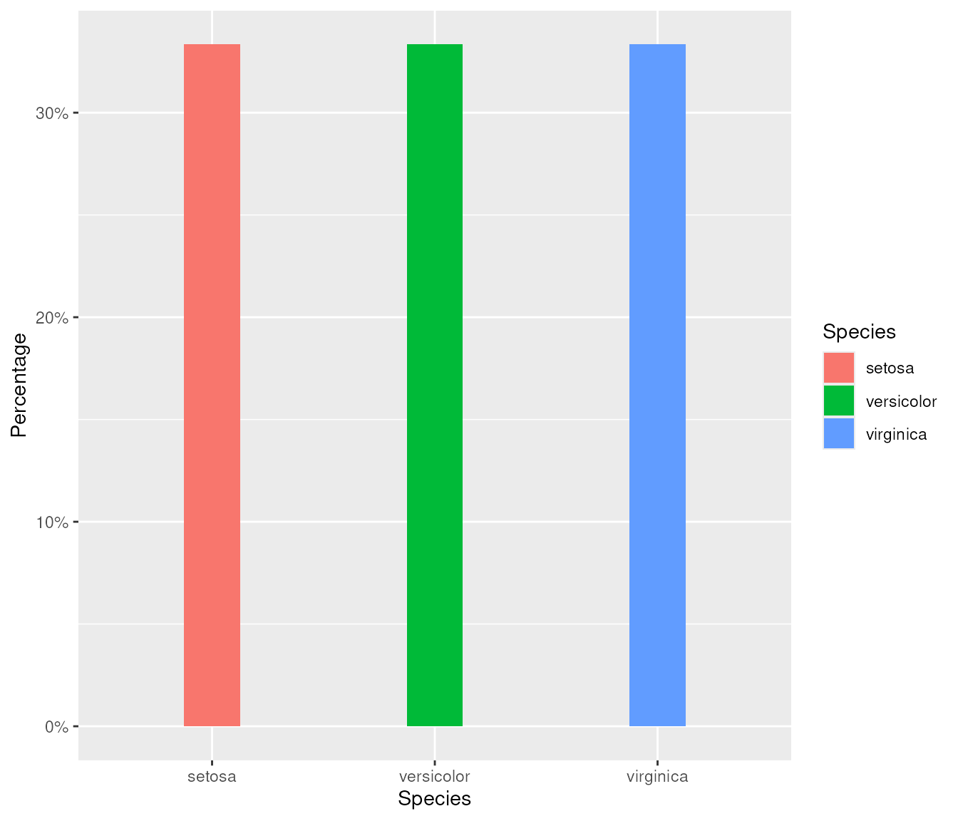

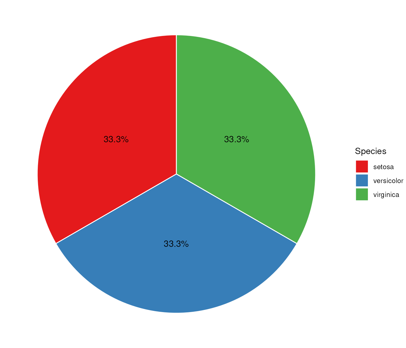
We can also use <percent> vectors as ggplot aesthetics¹

gg_data |>
  ggplot(aes(x = "", y = perc, fill = Species)) +
  geom_bar(stat = "identity", width = 1, color = "white") +
  coord_polar("y", start = 0) +
  theme_void() +
  geom_text(aes(label = perc), position = position_stack(vjust = 0.5)) +
  scale_fill_brewer(palette = "Set1")
#> Don't know how to automatically pick scale for object of type <percent>.
#> Defaulting to continuous.
#> Don't know how to automatically pick scale for object of type <percent>.
#> Defaulting to continuous.

Nick Christofides

Motivation

Creating percentages

Rounding

Rounding via as_percent + digits

Rounding via round()